As a CS Student, if you are studying Data Science, then the chances of encountering a Time-Series Forecasting Assignment are quite high. To work on such assignments, you have to build the “ARIMA Model in Python”.
Time-Series Forecasting is an important task as it has many real-world applications in the Stock Market, Sales, etc. And the ARIMA Model will be the best in such prediction fields. So, you must know about it.
If you’re working on an assignment and struggling to manage time-series forecasting. You can also check out our Python homework help guide for step-by-step support on common student problems.
In this article, we will give you a beginner-friendly tutorial to build and tune ARIMA models using Python for Time-Series Forecasting if you are working on a university assignment. So, let us start our discussion.
TL;DR: ARIMA Model In Python For Time-Series Forecasting
Aspect | Summary |
What Is ARIMA? | ARIMA is a statistical model used to forecast time-series data by analyzing past values and trends. |
ARIMA Stands For | Auto Regressive (AR), Integrated (I), Moving Average (MA) |
Required Python Packages | pandas, numpy, matplotlib, statsmodels, sklearn, pmdarima (optional). |
Steps Of ARIMA Building |
|
Outputs | ARIMA Model Summary, Model Evaluation Of 12 Months, 4 Graphs |
Model Evaluation | Performance is checked using Mean Absolute Error (MAE) and Root Mean Squared Error (RMSE). |
Important Tip | Always test for stationarity using the ADF test before applying ARIMA. |
What Is Time-Series Forecasting In Python?
Time-Series Forecasting is an assignment in Python where we analyze time-ordered data to predict the future. And the past patterns of the data help in this. Also, a variety of libraries and tools are used in this process.
Time-Series Forecasting is a very complicated assignment that can be divided into some steps, like preparing the data, choosing the right model, training it, and, in the end, getting the prediction from the code.
Some of the examples of Time-Series Forecasting can be predicting temperature for the next week, Forecasting sales for the next month, etc. To do Time-Series Forecasting, the ARIMA Model is highly used.
What Is The ARIMA Model In Python?
The ARIMA Model is one of the most commonly used models in Time-Series Forecasting. The ARIMA Model is developed on Mathematical Modeling, where the data’s past behavior is analyzed.
The ARIMA Model can only be implemented where the Time-series data is Stationary. That means, the Statistical Values like Mean and Variance are not changing with time.
If the Statistical Values are getting changed with time, the ARIMA will first make it Stationary. There are 3 powerful statistical techniques used to show the predictions. The ARIMA is an acronym that stands for:
- Auto Regressive (AR): This uses the past value of the data to predict the future of it.
- Integrated (I): This helps to make the data stationary by removing the trends from it.
- Moving Average (MA): If there are errors in the past predictions, those are used to improve forecasting.
What Are The Python Libraries Required To Build An ARIMA Model?
Now, if you are thinking of developing an ARIMA Model for Time-Series Forecasting, then you should have some Python Libraries installed on your system. Without these libraries, we can’t work with ARIMA.
In this section, we will inform you about the Python Libraries and their contributions to the Python ARIMA Model. So, let us check the following list to know more about such libraries in Python.
- Pandas: The Pandas are used to handle and manipulate the data given for the time series.
- NumPy: To do some numerical operations and array handling, the NumPy library is used.
- Matplotlib: In ARIMA, to draw the graphs and charts, the Matplotlib library is used.
- Seaborn: Seaborn works as an alternative to Matplotlib to create Statistical Graphs in ARIMA.
- Statsmodels: Statsmodels are used to build and tune the ARIMA model manually.
- Pmdarima (Optional): If you want to build the ARIMA Model automatically, then Pmdarima is used.
As such, Python Libraries are required to work with the Time-series ARIMA Model; we need to install them on the system. For the simultaneous installation of all packages, the following command can be used.
pip install pandas numpy matplotlib seaborn statsmodels pmdarima
How To Build And Tune An ARIMA Model For Forecasting Time Series?
As we have ample knowledge of time-series and ARIMA Models, it is time to build and tune the ARIMA Model from scratch. Don’t get worried, we will discuss that in a beginner-friendly manner.
The development of an ARIMA Model for Time-series forecasting can be divided into six steps. We will demonstrate each step, along with the corresponding code snippet and its explanation, to ensure a clear understanding.
Step 1: Importing The Necessary Libraries
To build the ARIMA Model, we have to first import the necessary libraries into the code. Without the imported libraries, we can’t move a single line in the program, and we will import a couple of packages.
Let us check the following code, where all the necessary packages are mentioned, which we have to import.
# Importing The Necessary Packages
import pandas as pd
import numpy as np
import matplotlib.pyplot as plt
from statsmodels.tsa.arima.model import ARIMA # This Package Will Implement The ARIMA
from statsmodels.tsa.stattools import adfuller # This Statsmodels Package Will Do ADF Test
# To End Model Evaluation
from sklearn.metrics import mean_absolute_error, mean_squared_error
# Packages To Remove Warnings From Code
import warnings
warnings.filterwarnings("ignore")
Explanation Of The Code:
- At first, the Pandas, NumPy, and Matplotlib Packages will be imported and will provide small names.
- Then, from the Statsmodels Package, we will import the ARIMA and Adfuller packages to do the ADF.
- For model evaluation, the Sklearn Package will be imported into the code.
- To remove some minor warnings from the output, we will use Warning Packages.
Step 2: Uploading The Data To Code
Now, the second thing that we have to do for the Forecasting Model is to upload the data. In this case, we will use the Monthly Sales Data for 5 Years, which will be uploaded to the program to work on it.
Once the data is loaded into the program, it can analyze the pattern and forecast the future outcomes.
# We Will Generate Monthly Sales Data For 5 Years
np.random.seed(42) # We Will Set The Seed For Reproducibility
# Creating The Monthly Dates
dates = pd.date_range(start=’2015-01-01’, periods=60, freq=’M’)
sales = np.cumsum(np.random.normal(loc=200, scale=50, size=len(dates))) + 5000
# Generating Sales Data With Upward Trend And DataFrame
df = pd.DataFrame({‘Date’: dates, ‘Sales’: sales})
df = df.set_index(‘Date’)
# Creating The Original Plot With Sales Data
plt.figure(figsize=(10, 4))
plt.plot(df[‘Sales’], label=’Sales’)
plt.title("Original Data For Monthly Sales")
plt.xlabel("Date")
plt.ylabel("Sales")
plt.grid(True)
plt.legend()
plt.show()
Explanation Of The Code:
- At first, Monthly Sales Data will be simulated using the Random Values.
- Now, a Cumulative Sum will be calculated from the Monthly Sales Data to show real-world trends.
- This data will be placed in a Dataframe that will be indexed using the Date and Sales.
- In the end, we will plot the Sales Data to show how it is evolving with time.
Step 3: Converting The Collected Data To Stationary
In the next step, we will convert the collected data to Stationary. Most real-world data is not stationary. So, we have to differentiate them to get the correct value. This is the most important step.
After that, we will do the Augmented Dickey-Fuller or ADF Test to check the stationarity status of the data.
# Converting Data To Stationary Using Differencing
df['diff'] = df['Sales'] - df['Sales'].shift(1)
# Creating The Differenced Data Plot
plt.figure(figsize=(10, 4))
plt.plot(df['diff'].dropna(), color='orange')
plt.title("Differenced Sales Data: ")
plt.xlabel("Date")
plt.ylabel("Differenced Sales")
plt.grid(True)
plt.show()
# Calculating The Augmented Dickey-Fuller (ADF) Test
result = adfuller(df['diff'].dropna()) # ADF Test Will Run On Differenced Series
print("ADF Statistic Is:", result[0]) # We Will Show The ADF Test Statistic
print("P-Value Will Be:", result[1]) # The P-Value Should Be Less Than 0.05
print("Critical Values Are:", result[4]) # Priting The Threshold Values
Explanation Of The Code:
- At first, we will subtract each sales value from its previous sales value for Differencing.
- Then, we will place all the data in a newly created column in the DataFrame.
- Later, the differenced data will be plotted, and the ADF Test will be performed.
- If the P-value in the ADF Test is less than 0.05, then the data is now Stationary.
Step 4: Build And Tune The ARIMA Model
Now, in this step, we will develop the ARIMA Model to work on the dataset that is not stationary. You can also term that we are manually building and tuning the ARIMA Model here for your easy understanding.
Let us check the following code, where the ARIMA Model is developed with a certain parameter.
# ARIMA Model Will Be Manually Developed
model = ARIMA(df[‘Sales’], order=(1,1,1)) # ARIMA model Will Have (P=1, D=1, Q=1)
model_fit = model.fit() # Providing The Original Data
print("\nARIMA Model Details: ")
print(model_fit.summary()) # Showing Summary With Coefficients, AIC, BIC, etc.
Explanation Of The Code:
- Here, the ARIMA Model will be developed with the parameter (p=1, d=1, q=1).
- Then, we will fit the original data or non-differenced data to the ARIMA Model.
- In the end, we will print the summary table to understand the model details.
Step 5: Forecasting The Time-Series
Now, the ARIMA Model is ready to forecast the future. It can read the past sales data and, based on it, it will predict the future. This prediction will be done by creating a graph using the Matplotlib Package.
The earlier sales data and the future sales data will all be plotted in a single graph for easy understanding.
# We Will Forecast The Next 12 Months Using The Trained Model
forecast = model_fit.forecast(steps=12) # Giving The Value 12 For 12 Months
forecast_index = pd.date_range(start=df.index[-1] + pd.DateOffset(months=1), periods=12, freq=’M’)
# Creating New Datetime Index
forecast_df = pd.DataFrame({‘Forecast’: forecast}, index=forecast_index)
# We Will Compare The Forecast Plot And Historical Data
plt.figure(figsize=(12, 6))
plt.plot(df[‘Sales’], label=’Historical Sales’)
plt.plot(forecast_df[‘Forecast’], label=’Forecast’, color=’red’)
plt.title(“Sales Forecast For 12 Months”)
plt.xlabel(“Date”)
plt.ylabel(“Sales”)
plt.grid(True)
plt.legend()
plt.show()
Explanation Of The Code:
- First, we will create a New Data Range for forecasting the future of the sales.
- Now, we will take 12 data points that will forecast the next 12 months of sales.
- The Historical Sales or Previous Sales and the Future Sales will all be plotted in the same graph.
Step 6: Evaluating The ARIMA Model
The last step is about the Evaluation of the ARIMA Model. In this step, we check how well our ARIMA Model is working. For that purpose, we split the last 12 months of data as the Test Set and then train it.
Here, we will calculate the Mean Absolute Error (MAE) and Root Mean Squared Error (RMSE) for the data.
# We Will Split The Data Into Training And Testing Sets
train = df['Sales'][:-12] # We Will Use All Data Except last 12 Months
test = df['Sales'][-12:]
eval_model = ARIMA(train, order=(1,1,1)).fit() # ARIMA Model Will Be Used On Training Data
preds = eval_model.forecast(steps=12) # Forecasting The Next 12 Months
# We Will Calculate The Model Performance Metrics
mae = mean_absolute_error(test, preds) # Mean Absolute Error
rmse = np.sqrt(mean_squared_error(test, preds)) # Root Mean Squared Error
print(f"\nModel Evaluation On Last 12 Months:")
print(f"Mean Absolute Error: {mae:.2f}")
print(f"Root Mean Squared Error: {rmse:.2f}")
# We Will Compare The Actual Plot And Predicted Data
plt.figure(figsize=(10, 5))
plt.plot(test.index, test.values, label="Actual", marker='o')
plt.plot(test.index, preds, label="Predicted", marker='x', color='red')
plt.title("Actual Vs Predicted Sales For Last 12 Months: ")
plt.xlabel("Date")
plt.ylabel("Sales")
plt.grid(True)
plt.legend()
plt.show()
Explanation Of The Code:
- First, we will split the data into a Training Set and a Test Set.
- The Training Set will have all data except the last 12 months, and the Test Set will have the last 12 months’ data.
- A New ARIMA Model will be trained on the training set and will forecast the next 12 months.
- Then, we have to compare the forecast with the actual test data using MAE and RMSE.
- Then, we have to draw a plot for the Actual and Predicted Values for better understanding.
What Will We Get As The Output Of Time-Series Forecasting?
After understanding the ARIMA Model for Time-series Forecasting, we have to move to its output. When we execute the entire code, we will get some outputs that we need to understand for analysis.
After executing the code, we will get 3 types of output. Let us check the output in the following.
1. ARIMA Model Summary:
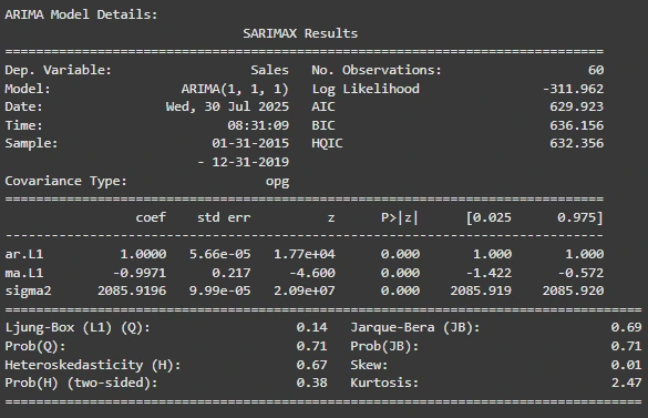
As we have developed the ARIMA Model in Step 4, we will get a summary table. This summary table will tell us the following things. Let us check those in the list below.
- The ARIMA Model is successfully fitted because it has a good score (AIC: 629.92, BIC: 636.15).
- There is no Autocorrelation and Normal Distribution in Residual Diagnostics (Ljung-Box, Jarque-Bera), which shows reliable predictions.
- The Stability of the model is confirmed by the Constant Variance in residuals (Heteroskedasticity Test)
2. Model Evaluation Of 12 Months:
The ARIMA Model Evaluation that we have done in Step 6 will also be printed on the output. From this output, we can understand the following things.
- The ARIMA Model performance was measured by the MAE (66.66) and RMSE (81.14).
- These error values show that forecasting was quite decent, and it is acceptable.
3. Graphs:
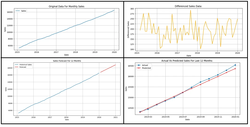
For the remaining steps in the ARIMA Model, we will get 4 graphs. Let us check those graphs and their details one by one from the following list.
- Original Data for Monthly Sales: This shows a steady upward trend for the actual sales data.
- Differenced Sales Data: The Transformed Sales Data after removing the trend is shown in this graph.
- Sales Forecast for 12 Months: The forecasted sales for the next year are mentioned in this graph.
- Actual Vs Predicted Sales: In this graph, we will compare the actual sales with predicted values.
Conclusion:
In the end, we can say, Time-series Forecasting with “ARIMA Model in Python” is not so complicated.
You have to just understand the six most important steps, and the rest you can do on your own. So, don’t get tensed after having such a complex assignment, and start with step 1 and create your project.
Takeaways:
- ARIMA Model stands for the Auto Regressive Integrated Moving Average.
- NumPy, Pandas, Matplotlib, Statsmodels, etc., are some important Python packages for ARIMA.
- There are six important steps to build and tune ARIMA for time series forecasting.
- Loading the data, converting to Stationary, Building ARIMA, Forecasting, and Evaluating are some steps.
- ARIMA Model Summary, Model Evaluation, and Graphs are some outputs in Forecasting.


