Understanding “Dijkstra’s Algorithm in C++” can be confusing at first, particularly for those who struggle with graphs, shortest paths, etc. Many students find it difficult to figure out how the algorithm actually works step by step.
It is even more challenging for students to convert that logic into working C++ code. The problem is not the syntax, but the lack of clarity in concepts like distance updates and node selection.
In this article, I will break down Dijkstra’s Algorithm simply and practically, so you can clearly understand the logic and confidently implement it in C++ for real-world problems. So, let us start.
TL;DR: Dijkstra’s Algorithm In C++
Aspect | Summary |
What It Is | Dijkstra’s Algorithm is a greedy algorithm used to find the shortest path in a weighted graph. It calculates the minimum distance from a source node to all other nodes. |
Core Idea | Always pick the unvisited node with the smallest distance and update its neighbors. This process is called relaxation and ensures optimal shortest paths. |
How It Works | Initialize distances, visit nodes step by step, and update paths using edge weights. The algorithm continues until all nodes are processed. |
Limitations | It does not work with negative edge weights because it assumes finalized distances. Using it in such cases can lead to incorrect results. |
Real-World Use | Used in GPS navigation, networking, and routing systems to find optimal paths. It helps solve real-world shortest path problems efficiently. |
What Is The Dijkstra’s Algorithm?
Dijkstra’s Algorithm is a Greedy Algorithm used to find the shortest path from a source vertex to all other vertices in a weighted graph with non-negative edge weights.
A graph is a non-linear data structure made up of vertices and edges, where edges may have weights representing cost or distance.
The algorithm starts from a source vertex, assigns it a distance of zero, and sets all other vertices to infinity. It repeatedly selects the vertex with the smallest tentative distance and updates the distances of its neighboring vertices if a shorter path is found.
This process continues until the shortest paths are determined. Dijkstra’s Algorithm is efficient and widely used, but it does not work with negative edge weights.
Important Terms Used In Dijkstra’s Algorithm:
- Source Vertex: This is the starting vertex from which the algorithm begins and computes the shortest paths to other vertices.
- Destination Vertex: It is the target vertex for which the shortest path from the source is determined. In Dijkstra’s Algorithm, shortest paths are typically computed from the source to all vertices, not just a single destination.
- Path: It is a sequence of vertices connected by edges, representing a route from the source to a destination. Different paths may have different total costs.
- Weights: There are the numerical values assigned to edges that represent cost, distance, or time. Dijkstra’s Algorithm requires all edge weights to be non-negative.
Before learning Dijkstra’s algorithm, it is helpful to understand how data structures like trees and graphs are explored. Concepts like visiting nodes step by step are similar to what you see in Tree Traversal Techniques, which build a strong base for understanding such algorithms.
What Are The Steps Of Dijkstra’s Algorithm?
When you first learn Dijkstra’s Algorithm, you may feel it a bit technical, but the core idea is actually very simple, which states to always move to the closest unvisited node.
As someone who has taught this for years, I tell students to think of it like finding the shortest route on Google Maps step by step. If you follow the process carefully, you will never get confused, even in complex graphs.
Let us go through the simple and practical algorithm steps mentioned below.
- Start by assigning a distance value of 0 to the source node and infinity to all other nodes because we don’t know their shortest path yet.
- Create a visited set to keep track of nodes whose shortest distance is already finalized.
- Pick the node with the minimum distance and mark it as visited because now its shortest path is confirmed.
- For each neighbor of this node, calculate the new possible distance.
- If this new distance is smaller than the previously stored value, update it immediately.
- Repeat this process until all nodes are visited or the destination node is reached.
- At the end, the distance array will give you the shortest path from the source to every node.
Dry Run: Working Of Dijkstra’s Algorithm
Over the years, I have seen that students only gain true confidence when they trace Dijkstra’s algorithm step by step on a small graph. This is where the Dry Run concept plays an important role.
When you really want to master Dijkstra’s Algorithm, doing a dry run is not optional; it is essential. Think of this as manually simulating how the algorithm “thinks” while finding the shortest path.
To make you understand the working easily, I have broken it up into some effective steps. Let us check them.
Step 1: Initialization
We begin by selecting a source vertex. In this example, we choose A as the starting node. Since this is our starting point, we assign its distance as 0.
For all other nodes, which are B and C, we assign a distance of infinity because we haven’t discovered any paths to them yet. At this stage, none of the nodes are visited.
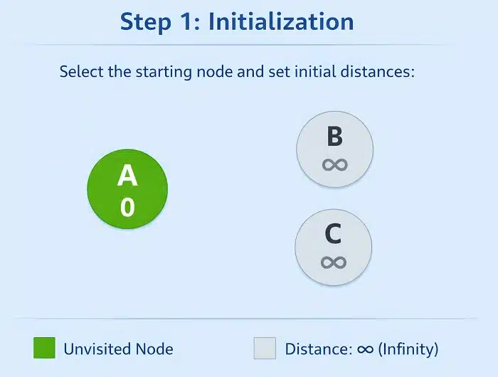
So, we maintain a clear separation between visited and unvisited nodes. Right now, all nodes are unvisited, and we are ready to start processing from node A.
Step 2: Visit Current Node And Update The Neighbors
Now, we start with node A because it has the smallest distance (0). We mark A as visited since we are now processing it. Next, we look at all its neighboring nodes, which are B and C.
The key idea here is to check whether we can reach these neighbors with a shorter distance through A. This process is called relaxation. For example, if the edge from A to B has a weight of 2, and A to C has a weight of 5, we update their distances accordingly.
So now, B gets a distance of 2, and C gets a distance of 5. This means we have found better paths to these nodes through A.
Step 3: Choose The Next Closest Node
At this point, we do not randomly pick the next node. Instead, we carefully select the unvisited node with the smallest distance value. Between B and C, node B has the smaller distance (2), so we pick B next.
We mark B as visited and repeat the same process. Now, we look at B’s neighbors and check whether going through B provides a shorter path to any node.
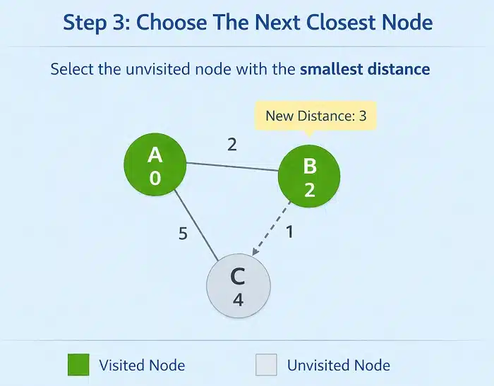
If there is a path from B to C, we calculate the new distance and compare it with the current distance of C. If it is smaller, we update it. This step is crucial because it ensures that we are always moving in the direction of the globally shortest path, not just the locally shortest edge.
Step 4: Process The Remaining Node
Now, only C remains unvisited. Since it is the only node left, we select it and mark it as visited. At this point, all nodes have been processed. There are no more nodes left to explore, and the algorithm terminates.
By now, we have already calculated the shortest distances from the source node A to all other nodes.
Dijkstra’s algorithm relies heavily on selecting the minimum distance node at each step. This process is often implemented using a Priority Queue, which helps efficiently pick the next node with the smallest distance.
How To Implement The Dijkstra’s Algorithm in C++?
Once your concepts are clear, implementation becomes much easier and more intuitive. So, in this section, I will let you know the implementation process of Dijkstra’s algorithm in C++.
For that purpose, I have prepared the following graph. On this graph, we have to apply Dijkstra’s algorithm. We will assume Node A is the starting point and figure out the distance of the other nodes from it using the algorithm.
If you focus on writing clean logic step by step, your C++ implementation will be both efficient and interview-ready.
#include
#include
using namespace std;
// Function to find the vertex with the minimum distance value
int minDistance(int dist[], bool Tset[]) {
int min = INT_MAX, min_index;
for (int i = 0; i < 6; i++)
if (Tset[i] == false && dist[i] <= min)
min = dist[i], min_index = i;
return min_index;
}
// Function to print the output
void output(int dist[]) {
cout << "Vertex \t Distance from the Source\n";
for (int i = 0; i < 6; i++){
char ver = 65+i;
cout << ver << " \t\t " << dist[i] << endl;
}
}
void dijkstraAlgorithm(int graph[6][6], int src) {
int dist[6]; // creating a list to store the shortest distances for each vertex
bool Tset[6];
for (int i = 0; i < 6; i++)
dist[i] = INT_MAX, Tset[i] = false;
dist[src] = 0; // this is because the distance from source to source is zero
// Finding shortest paths for each vertex
for (int count = 0; count < 6 - 1; count++) {
int u = minDistance(dist, Tset);
// Mark the vertex as visited
Tset[u] = true;
for (int v = 0; v < 6; v++)
if (!Tset[v] && graph[u][v] && dist[u] != INT_MAX && dist[u] + graph[u][v] < dist[v])
dist[v] = dist[u] + graph[u][v];
}
// Print the output
output(dist);
}
int main()
{
/* Let us create the example graph discussed above */
int graph[6][6] = { { 0, 1, 2, 0, 0, 0},
{ 1, 0, 1, 0, 3, 0},
{ 2, 1, 0, 2, 2, 0},
{ 0, 0, 2, 0, 1, 1},
{ 0, 3, 2, 1, 0, 2},
{ 0, 0, 0, 1, 2, 0},
};
dijkstraAlgorithm(graph, 0);
return 0;
}
Steps Of The Program:
- In the above code, we see that we have a graph that has six vertices named from A to F.
- The weights on these are also mentioned. The whole graph is represented in the main() as graph[6][6]
- Now, we pass this graph as an argument to the function dijkstraAlgorithm() that firstly marks all these vertices as unvisited by setting the shortest path tree (Tset) as false.
- Then we take up each vertex one by one and start calculating the distance and updating the distance in the array dist.
- When the whole operation is completed, we print the shortest path from the source of all vertices using the output() function.
Output:
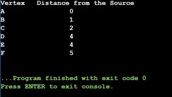
From the above output, we can see all the shortest paths from vertex A to other vertices in the graph. We see that the distance from vertex A is 0, as it is the source vertex. As we move to the other vertices, we can see how adding the weights on the paths gives us the final shortest distance.
What Are The Time And Space Complexities Of C++ Dijkstra’s Algorithm?
As I am mentoring students in DSA for decades, I can tell you that in real-world systems and coding interviews, the Time and Space Complexities become more important than just writing correct code.
Understanding these complexities is important because it tells you whether your solution will scale for large inputs. Let us break down the time and space complexities in a way that you can easily remember.
Time Complexity:
If you are using a priority queue or min-heap, the time complexity is O((V + E) log V)
Here, the V is the number of vertices (nodes), E is the number of edges, and the (log V) factor comes from heap operations like insertion and extraction.
Space Complexity:
The space complexity will be O(V + E). The space complexity includes the Graph storage (adjacency list), Distance array, and Priority queue.
Comparison Table Between Dijkstra, BFS, And Bellman-Ford Algorithms:
Many times, students ask me that they are getting confused between Dijkstra’s Algorithm, Breadth-First Search (BFS), and the Bellman-Ford Algorithm, as they all are used to find paths in a graph.
In such cases, I have to draft a comparison table between them to clarify the confusion. When you compare these algorithms, you start seeing when to use which one; this is where real understanding comes in.
Criteria | Dijkstra Algorithm | BFS Algorithm | Bellman-Ford Algorithm |
Graph Type | Weighted | Unweighted | Weighted |
Negative Weights | No | No | Yes |
Data Structure | Heap | Queue | None |
Time Complexity | Fast | Fast | Slow |
Approach | Greedy | Level | Relaxation |
Cycle Handling | Yes | Yes | Yes |
Use Case | Shortest | Shortest | General |
Why Dijkstra’s Algorithm Fails For Negative Weights?
Since I have been mentoring students for a long time, I have seen this important conceptual question often comes in exams, and many students misunderstand it and lose points. That is why I am clearing it here.
Dijkstra’s Algorithm works perfectly, but under only one condition, which is that all edge weights must be non-negative. If you break this rule, the algorithm can give wrong answers without any warning.
Here is the intuition you should never forget to answer this question:
- Dijkstra’s Algorithm assumes that once a node is visited, its shortest distance is final.
- This assumption completely breaks when negative weights are present.
Suppose you have already finalized a node with a distance of 5. Later, you find another path reaching the same node with distance 3 using a negative edge. But Dijkstra will never reconsider that node, so it keeps the wrong value (5).
If I break down the answer in simpler terms, the following points come. These points you should memorize.
- Negative weights can create shortcuts after a decision is already made.
- Dijkstra does not backtrack, so it misses these better paths.
That is why for graphs with negative weights, we use the Bellman-Ford Algorithm, which safely relaxes edges multiple times.
What Are The Real-World Applications Of The Dijkstra’s Algorithm?
When students ask me where Dijkstra’s Algorithm is actually used, I always say it is far more practical than it looks in textbooks. This algorithm is quietly working behind many systems you use every day.
Once you understand its applications, you will start seeing Dijkstra’s Algorithm as a real-world problem solver, not just a coding concept. That is why I love to share the real-world applications of it with students. Here is the list.
- Dijkstra’s Algorithm C++ is highly used in the computer networking concept to find the nearest node present that helps to work routers & other internet gadgets.
- This algorithm helps to find out the shortest distance between two locations, which helps to develop different map applications in Android or web browsers. Dijkstra’s Algorithm is used in GPS systems, mapping of geological locations, and IP routing.
- Dijkstra’s Algorithm C++ helps to find the nearest switching station in the telephonic conversation process, which helps to connect one device to another easily.
- This algorithm is used to find possible hops present in a computer network. And if they are present, it helps to reduce the count in the computer networking.
- Dijkstra’s Algorithm C++ helps to find out the shortest path present in between the handshake method or the connection build-up with the help of that method. Simply, it helps in electronic engineering.
Common Mistakes Students Make With Dijkstra’s Algorithm In C++:
When students start learning Dijkstra’s Algorithm in C++, most mistakes do not come from syntax, but from misunderstanding how the algorithm actually works.
From my experience mentoring students, many of them try to “shortcut” the logic and end up writing code that looks correct but gives wrong results.
One very common mistake I see is that students treat Dijkstra’s algorithm like a simple traversal and directly mark nodes as visited without maintaining the shortest distance properly. An incorrect implementation often looks like this:
// Incorrect approach: Treating it like BFS
visited[u] = true;
for (auto v : adj[u]) {
if (!visited[v]) {
dist[v] = dist[u] + 1; // assumes equal weights
q.push(v);
}
}
This approach is wrong because Dijkstra’s Algorithm does not assume equal weights and should not rely on a normal queue like BFS. It also ignores the idea of updating a node if a shorter path is found later.
Now, if we correct this and follow the proper logic using a priority queue, the implementation becomes:
// Correct approach using priority queue
priority_queue, vector>, greater<>> pq;
pq.push({0, source});
dist[source] = 0;
while (!pq.empty()) {
auto [d, u] = pq.top();
pq.pop();
}
Here, we always process the node with the smallest distance first, which is the core idea behind Dijkstra’s Algorithm. Along with this, there are several other common mistakes that I frequently notice in student implementations:
- Students forget to update the distance properly using relaxation and simply assign values without comparison.
- Many students do not use a priority queue (min-heap) and instead use a normal queue, which breaks the algorithm logic.
- Sometimes, students mark a node as visited too early, without confirming that the shortest path to that node is finalized.
- I have seen students ignore edge weights or assume all weights are equal, which makes their solution behave like BFS instead of Dijkstra.
- Students often forget that Dijkstra’s Algorithm does not work with negative edge weights, and still try to apply it in such cases.
Conclusion:
By now, you should have a clear understanding of how “Dijkstra’s Algorithm in C++” works and how to implement it step by step.
Once you are comfortable with this concept, you will be able to solve a wide range of shortest path problems with confidence, which is a big step forward in your DSA journey.
If you are learning algorithms, it is useful to explore different problem-solving approaches. While Dijkstra’s algorithm focuses on shortest paths, sorting techniques like the Quick Sort Algorithm help you understand how data can be arranged efficiently in different scenarios.
Key Takeaways:
- Dijkstra’s Algorithm is one of the algorithms in the group of greedy algorithms.
- These algorithms help us to make the optimal choices at the local or current stage.
- Dijkstra’s Algorithm works in a graph having positive weights. It is used to calculate the shortest distance between two points.
- The point from where the algorithm starts is the source vertex, and the other point is the destination vertex.
- In C++, Dijkstra’s Algorithm helps us to find the shortest path from one source to all the other vertices in the graph.
- This algorithm is used in GPS systems, mapping of geological locations, and IP routing.
Frequently Asked Questions:
1) Can Dijkstra’s Algorithm be used for directed graphs?
Yes, it works perfectly for both directed and undirected graphs. The only requirement is that all edge weights must be non-negative. Direction of edges is naturally handled through the adjacency list.
2) Is Dijkstra’s Algorithm suitable for dense graphs?
It can be used, but performance may degrade due to a large number of edges. In dense graphs, the number of edge relaxations increases significantly. Other approaches or optimizations may be considered depending on constraints.
3) Can Dijkstra’s Algorithm handle cycles in a graph?
Yes, it can handle cycles as long as there are no negative-weight edges. The algorithm ensures that nodes are processed based on the shortest distance. Cycles do not affect correctness because distances are only updated when shorter paths are found.


